Thermal Management & Cold Plate Design

Key Engineering Contributions

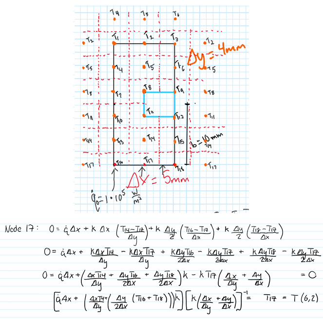
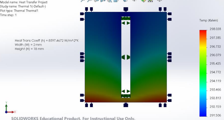
1. 01
   Thermal System Design: Designed the internal architecture of a water-cooled cold plate to effectively dissipate a uniform heat flux of 105 W/m2 generated by the simulated electronic components.
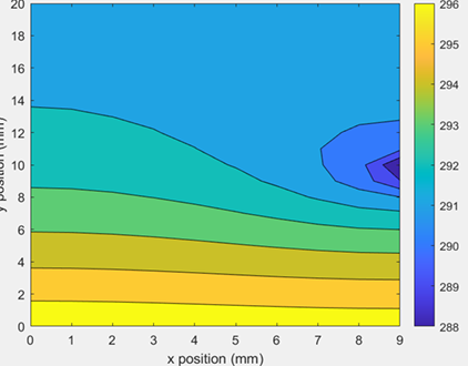
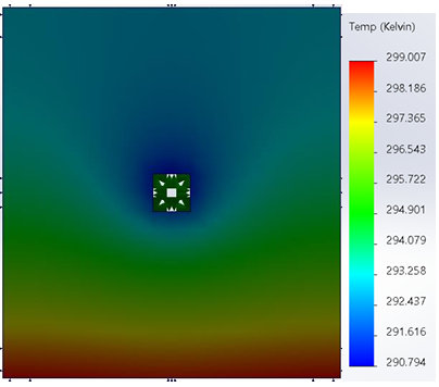
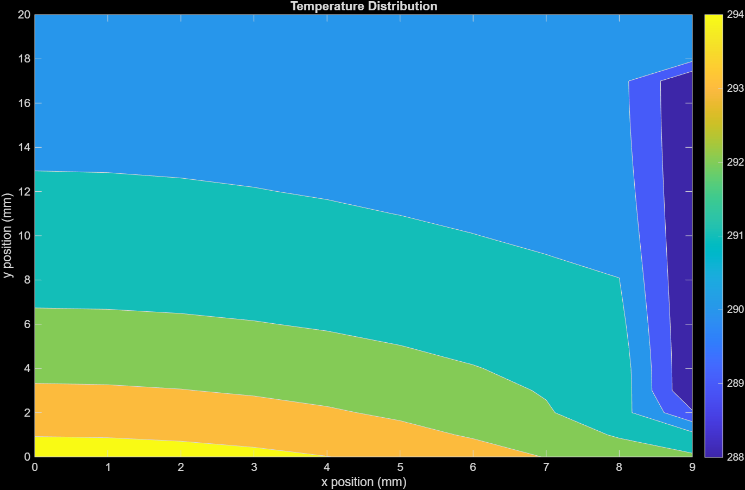
2. 02
   Computational Heat Transfer (FEA): Conducted rigorous thermal simulations in MATLAB and SolidWorks to model the heat conduction through the aluminum substrate and the forced convection into a 15°C internal water flow.
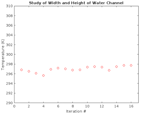
3. 03
   Analytical Fluid Modeling: Developed mathematical algorithms in MATLAB to compute the Reynolds Number, convective heat transfer coefficient (h) across varying internal channel geometries, and temperature distribution optimizing the design for maximum thermal efficiency.

Visual Documentation

Figure 1

01.png

Sample calculation of a node based on 2-D heat transfer principal equations (energy balance). These conditions are of different spacing than the code used in the MATLAB program as the nodes are much c

Figure 2

02.png

Contour Plot made in MATLAB of the study of the water channel’s dimensions at a width of 2mm and a height of 2 mm with nodes spaced evenly, 𝛥𝑥 = 1𝑚𝑚 and 𝛥𝑦 = 1𝑚. The MATLAB program calculates the wate

Figure 3

03.png

SolidWorks simulation contour plot of thermal analysis of square channel with a width and height of 2mm. SolidWorks utilizes calculated heat transfer coefficients from MATLAB to confirm the program’s

Figure 4

04.png

MATLAB dot plot of one of multiple parametric studies to optimize the design with respect to thermal performance. This specific study examines the maximum temperatures at 16 different width and height

Figure 5.1

05-1.png

Part 1 of 2

Figure 5.2

05-2.png

Part 2 of 2