Index / Work / N° 04
Project N°04 of 24
CategoryRobotics · Control
Year2025

Adaptive Control & Estimation for Wearable Exoskeletons

Engineered and evaluated multiple assistive control architectures to minimize human exertion within a provided Simulink model of a 1-DOF hip exoskeleton and human leg.

Key Engineering Contributions

  1. 01
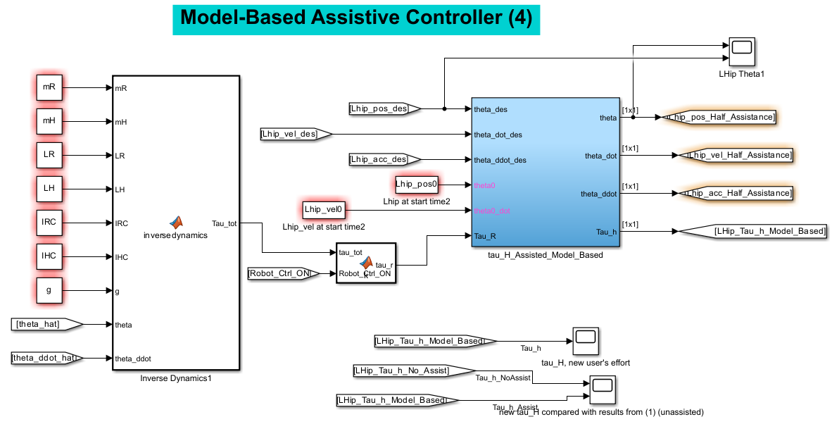
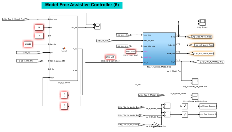
    Control System Integration: Analyzed a provided Simulink baseline simulation of human gait dynamics and successfully integrated custom controller subsystems to assist the simulated treadmill walking trajectory.
  2. 02
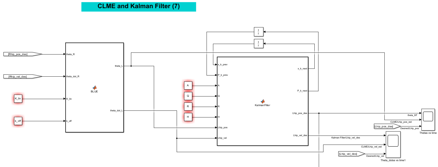
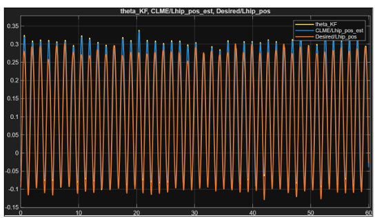
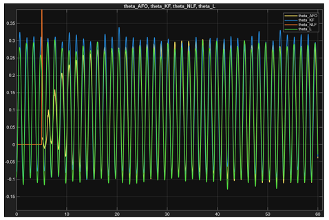
    State Estimation & Filtering: Utilized Best Linear Unbiased Estimators (BLUE) to process baseline kinematic data and implemented a Kalman Filter to estimate hip trajectories under noisy biomechanical conditions.
  3. 03
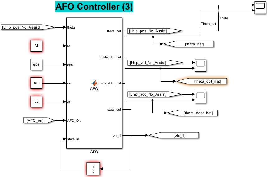
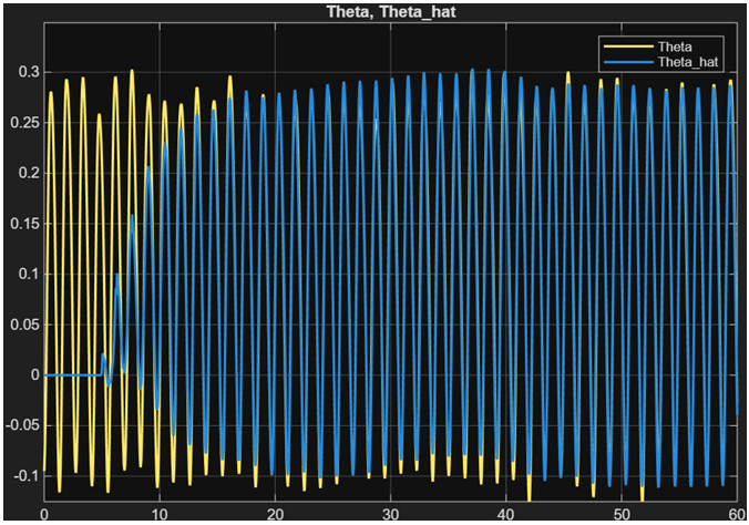
    Adaptive Control Design: Formulated the initial conditions and tuned an Adaptive Frequency Oscillator (AFO) control scheme to actively synchronize with the user's rhythmic gait and provide real-time assistive torque.
  4. 04
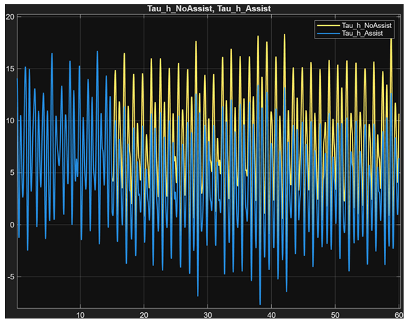
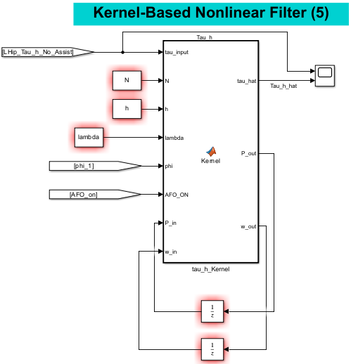
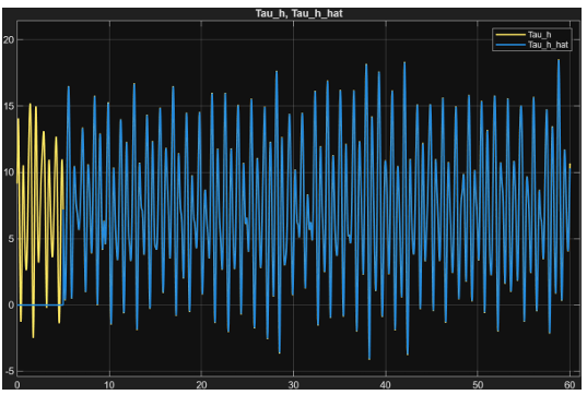
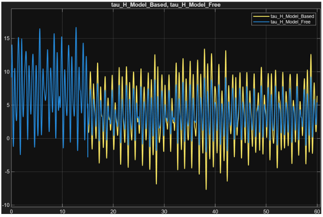
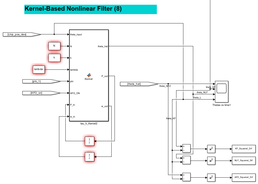
    Advanced Nonlinear Control: Engineered a custom Kernel-Based Nonlinear Filter (NLF) that successfully outperformed the traditional linear estimators, achieving the highest tracking accuracy with a Root Mean Square (RMS) error of just 0.0178.

Visual Documentation

Model of the hip exoskeleton and human leg
Figure 1
01.png
Model of the hip exoskeleton and human leg
The left figure shows the adaptive frequency oscillator (AFO) controller Simulin (image 1 of 2)
Figure 2.1
02-1.png
Part 1 of 2
The left figure shows the adaptive frequency oscillator (AFO) controller Simulin (image 2 of 2)
Figure 2.2
02-2.png
Part 2 of 2
The left figure shows the adaptive frequency oscillator (AFO) controller Simulink setup. The right plot displays actual hip angles (yellow) and the estimated hip angle from the AFO (blue) (with respect to time). The plot confirms accuracy.
The left figure shows the model-based assistive controller Simulink setup. The r (image 1 of 2)
Figure 3.1
03-1.png
Part 1 of 2
The left figure shows the model-based assistive controller Simulink setup. The r (image 2 of 2)
Figure 3.2
03-2.png
Part 2 of 2
The left figure shows the model-based assistive controller Simulink setup. The right plot displays human torque during unassisted walking (yellow) and human torqued during model-based assistive walking (blue). The plot shows much lower peaks in torque during assisted walking.
The left figure shows the kernal-based nonlinear filter controller Simulink setu (image 1 of 2)
Figure 4.1
04-1.png
Part 1 of 2
The left figure shows the kernal-based nonlinear filter controller Simulink setu (image 2 of 2)
Figure 4.2
04-2.png
Part 2 of 2
The left figure shows the kernal-based nonlinear filter controller Simulink setup. The right plot displays actual hip angles (yellow) and the estimated hip angle from the the kernal-based filter (blue) (with respect to time). The plot confirms accuracy.
The left figure shows the model-free assistive controller Simulink setup. The ri (image 1 of 2)
Figure 5.1
05-1.png
Part 1 of 2
The left figure shows the model-free assistive controller Simulink setup. The ri (image 2 of 2)
Figure 5.2
05-2.png
Part 2 of 2
The left figure shows the model-free assistive controller Simulink setup. The right plot displays assisted torque over time utilizing the model-based controller (yellow) and the model-free controller (blue) with respect to time. The assistance begins at ~15 seconds. The plot shows the model-free controller does a drastically better job at tracking the desired torque profile.
Simulink setup of complementary limb motion estimation (CLME) and Kalman fliter
Figure 6
06.png
Simulink setup of complementary limb motion estimation (CLME) and Kalman fliter Simulink setup. CLME approximates the left hip joint angle and angular velocity based on inputs from the right hip state
Simulink setup of complementary limb motion estimation (CLME) and Kalman fliter Simulink setup. CLME approximates the left hip joint angle and angular velocity based on inputs from the right hip state using a best linear unbiased estimator (BLUE). BLUE is trained using data from the first 30 seconds of the right and left hip trajectories. The training results in linear mapping and offset values to estimate the left hip state based on the right hip state. However, the resulting angular positions and velocities are not coherent. Therefore, a Kalman filter is required to adjust the output of BLUE to make the estimated state coherent.
Plot of desired/actual left hip angle (orange), the estimated left hip angle fro
Figure 7
07.png
Plot of desired/actual left hip angle (orange), the estimated left hip angle from CLME (blue), and the estimated left hip angle after the Kalman Filter (yellow) is applied with respect to time.
The left figure is the kernel-based nonlinear filter (NLF) Simulink setup. The r (image 1 of 2)
Figure 8.1
08-1.png
Part 1 of 2
The left figure is the kernel-based nonlinear filter (NLF) Simulink setup. The r (image 2 of 2)
Figure 8.2
08-2.png
Part 2 of 2
The left figure is the kernel-based nonlinear filter (NLF) Simulink setup. The right plot is the resulting NLF (orange), AFO (yellow), Kalman filter (blue), and desired hip angles. It is important to note that the spike non-linear filter’s estimated theta value of around 5 seconds is a result of initial conditions from its previous torque use. The most accurate of the estimations was that produced by the nonlinear Filter.